How to Visualize the NSD Dataset with Pycortex?

This blog is a tutorial on visualizing the Natural Scenes Dataset (NSD) with Pycortex, aimed at researchers who want a practical guide for neural data visualization.

Contents

• Preface
• I. Introduction to the NSD Dataset
• II. Introduction to the Pycortex Library
• III. Prerequisite Files
  • 1. Original Data to be Mapped
  • 2. Surface Database
• IV. Visualization Workflow
  • 1. Core Visualization Code
  • 2. ROI Labeling
• V. Public Release of the NSD Dataset Surface Database
• VI. Common Issues
  • 1. Flatmap Rotated by 90°
  • 2. Flatmap Sulcus/Gyrus Settings
  • 3. Defining ROIs with Inkscape via XLaunch
  • 4. Visualization Methods for Other Datasets Beyond NSD

• Reference

Preface

The Natural Scenes Dataset is an incredible resource — tons of high-quality fMRI data that’s just waiting to be explored. But if you’ve ever tried working with it, you’ll know the first hurdle: how exactly are neural activities (or other brain-related metrics) distributed across the cortex? And is there a way to visualize them in an intuitive way?

That’s where Pycortex comes in. With just a bit of setup, it lets us map NSD data onto cortical surfaces and create beautiful flatmaps (and even 3D views). In this post, I’ll walk through the process I used — from setting up the necessary files, to running the core visualization code, to adding ROIs, and even handling some common gotchas along the way.

Hopefully, this guide will save you some time (and headaches) if you’re diving into NSD visualization yourself. 😊🌱

I. Introduction to the NSD Dataset

The NSD dataset (Natural Scenes Dataset) is a large-scale, high-quality neuroimaging resource. Using high-resolution functional magnetic resonance imaging (fMRI), the research team recorded the neural responses of 8 participants while they performed a continuous recognition task on 73,000 natural scene images. These images come with rich annotations and are supplemented with resting-state and diffusion imaging data.

Paper: A massive 7T fMRI dataset to bridge cognitive neuroscience and artificial intelligence | Nature Neuroscience
Dataset homepage: Natural Scenes Dataset

Without further ado—if you want to download the data (⚠️ it is not recommended to blindly download everything, as the dataset is extremely large; it’s better to selectively download based on your needs), you can either follow the official guide NSD: How-to-get-the-dataor directly use the following method on your server:

1. Visit the AWS S3 public directory: AWS S3: natural-scenes-dataset.
   This is the open file directory for NSD on AWS S3, accessible without an AWS account.
   There are 7 folders in total. Each folder’s meaning is explained in NSD: Overview-of-the-data. You can choose which subsets to download depending on your needs.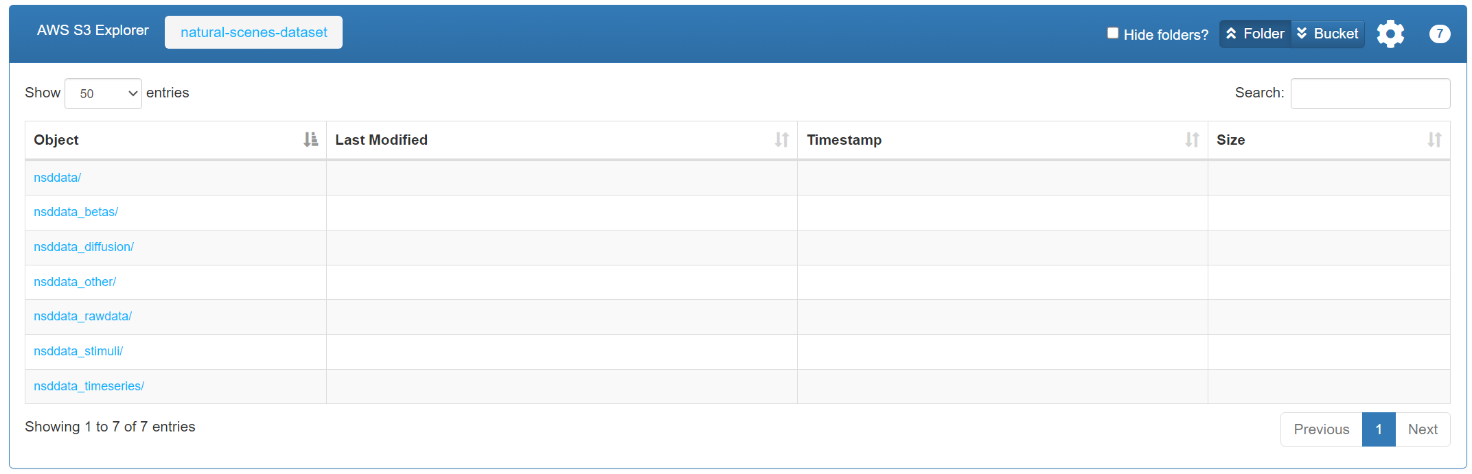

2. Once you’ve decided which subset(s) to download, run the following command on your server (for example, downloading s3://natural-scenes-dataset/nsddata_betas/ppdata/ into your local path YOURPATH). Thanks to the --no-sign-request flag, no AWS account is required.

#!/bin/bash

aws s3 sync --no-sign-request s3://natural-scenes-dataset/nsddata_betas/ppdata/ /YOURPATH
# aws s3 sync: use the AWS CLI to synchronize files from an S3 bucket to a local directory
# --no-sign-request: access public data without requiring an AWS account or credentials

At this point, the dataset has been successfully downloaded from AWS S3 to your server. It is worth emphasizing again that, due to the dataset’s enormous size (some folders are measured in terabytes), it is highly recommended to download only the files you need rather than attempting to download everything.

II. Introduction to the Pycortex Library

Pycortex is an open-source software package for fMRI data visualization. It allows you to project brain activity (or any other metric you want to visualize) onto a cortical surface model, generating interactive 3D visualizations. It also supports high-quality 2D flattened cortical maps.

Pycortex documentation: https://gallantlab.org/pycortex/. This documentation provides very detailed instructions on installation, usage examples, API references, and all other details. If you want to learn Pycortex in depth, you can directly study the documentation.

The following visualization workflow mainly focuses on 2D flattened cortical maps, also known as flatmap visualization. The core method is to map your data (i.e., the metric you want to visualize) onto a 2D cortical vector map, ultimately producing a result like the figure below. Note that in this demonstration figure, random data is used, which is why it appears very messy.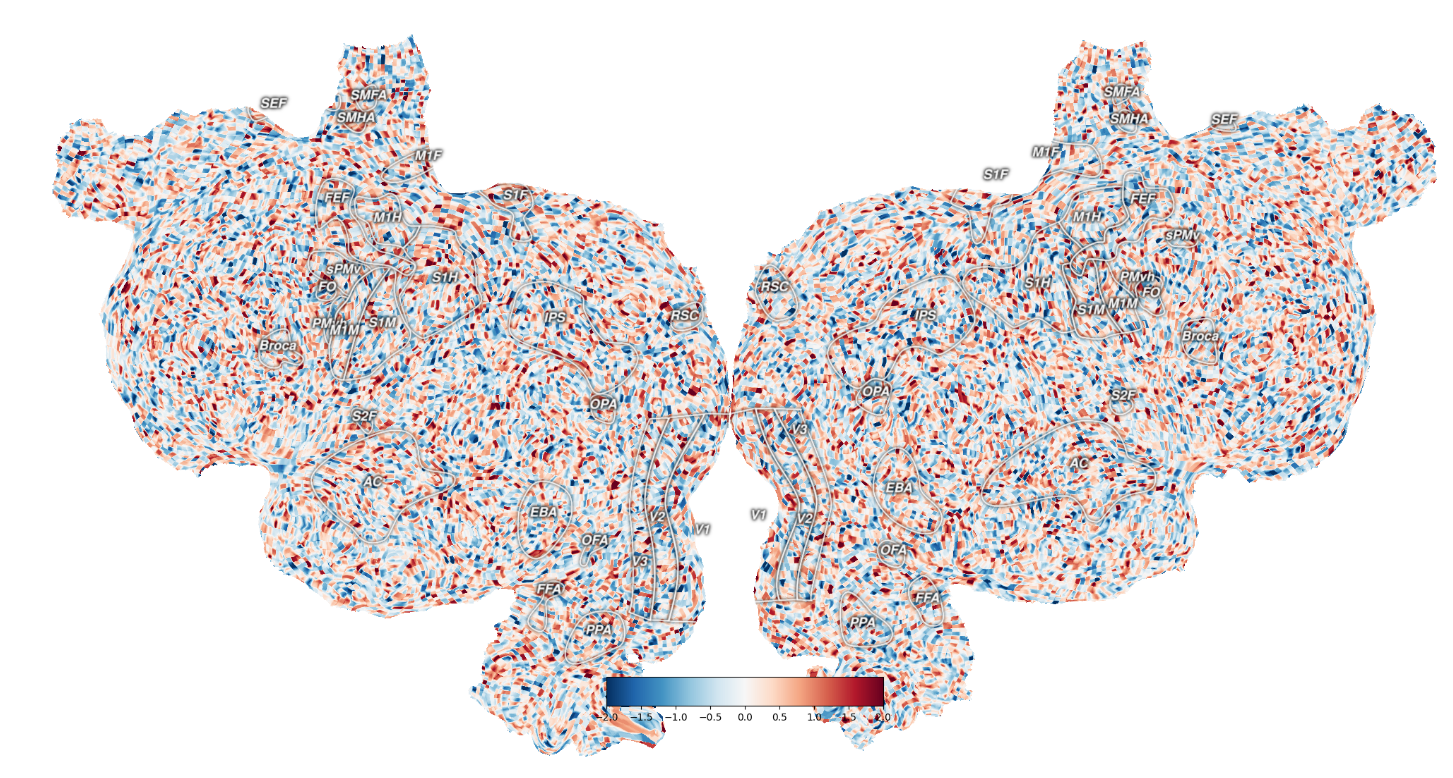

III. Prerequisite Files

Now, to clarify, if you want to perform flatmap visualization for the NSD dataset using Pycortex, the core method is to map your data (i.e., the metric you want to visualize) onto a 2D cortical vector map. Therefore, the required prerequisite files include: the raw data to be mapped and the Surface Database (the latter is a flat-file system used to manage and store all relevant files and information necessary for projecting data onto the cortical surface).

1. Original Data to be Mapped

First, it is important to understand that fMRI data is recorded at the voxel level. A voxel is the smallest unit of volume in 3D space, similar to a pixel in a 2D image, but with volume. Each voxel corresponds to a certain volume of neural tissue in the brain. Typically, a participant’s voxel data is organized into a 3D matrix of shape (H, W, B).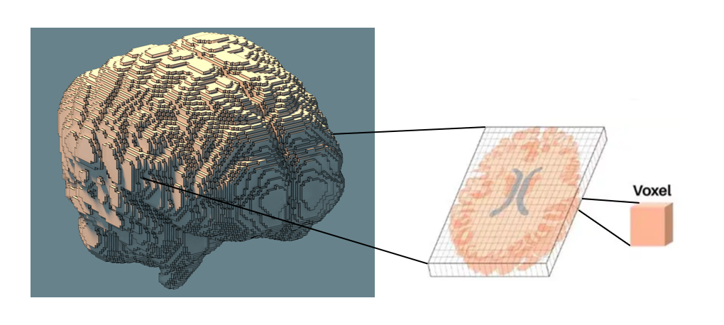

For each participant in the NSD dataset, the total number of voxels across the whole brain may vary due to inter-subject differences. Therefore, if we want to plot a flatmap for a specific participant corresponding to a certain metric, we must ensure that the matrix for that metric has exactly the same size as the original voxel matrix. But what exactly is the size of the original voxel matrix? And if we fail to ensure the sizes match during visualization, how is it detected? The answer lies in the Surface Database.

Returning to the main point of this tutorial, if we want to use Pycortex to visualize NSD participants via flatmaps, how do we obtain the corresponding database for each participant (Subj01–08)? Before discussing the specific methods for obtaining the surface database, let’s first provide a more detailed introduction to it.

2. Surface Database

The Surface Database is a flat-file system used to manage and store all relevant files and information needed to project data onto the cortical surface, including surface geometry, transformation matrices, ROIs, masks, and more.

In short, the database is essential to know how to map the raw data onto the 2D cortex to generate a flatmap and in what format the resulting flatmap will appear. For a single participant, e.g., S1, a complete database should include the following files. As you can see, the required files are quite complex. For detailed explanations of each file and its purpose, refer to the official documentation: Pycortex Documentaion: overlays-svg, which provides very thorough descriptions.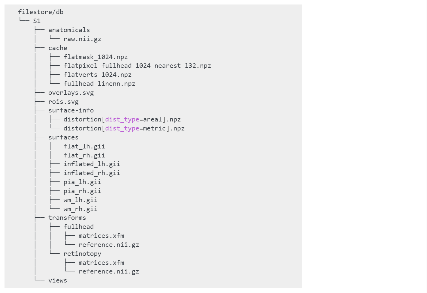

And thanks to the great NSD dataset contributors and Pycortex’s built-in functions, we can easily obtain the database corresponding to each participant. The specific workflow is as follows:

1. First, download the folders subj01–subj08 from AWS S3: natural-scene-dataset/nsddata/freesurfer to the directory /home/YOURNAME/freesurfer/subjects/.
   Note: There are many tutorials available for installing FreeSurfer, so we will not cover installation details here.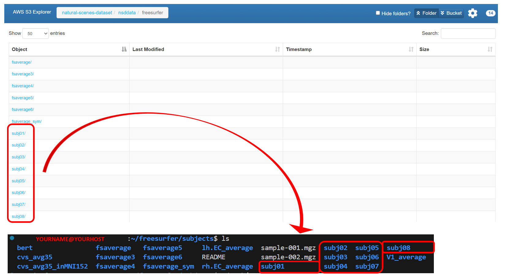

2. Download meanbeta.nii.gz for each participant from AWS S3: natural-scenes-dataset/nsddata_betas/ppdata under the path subj0X/func1pt8mm/betas_fithrf_GLMdenoise_RR/ to your server directory /YOURPATH. This data will be used as the reference fMRI file for alignment.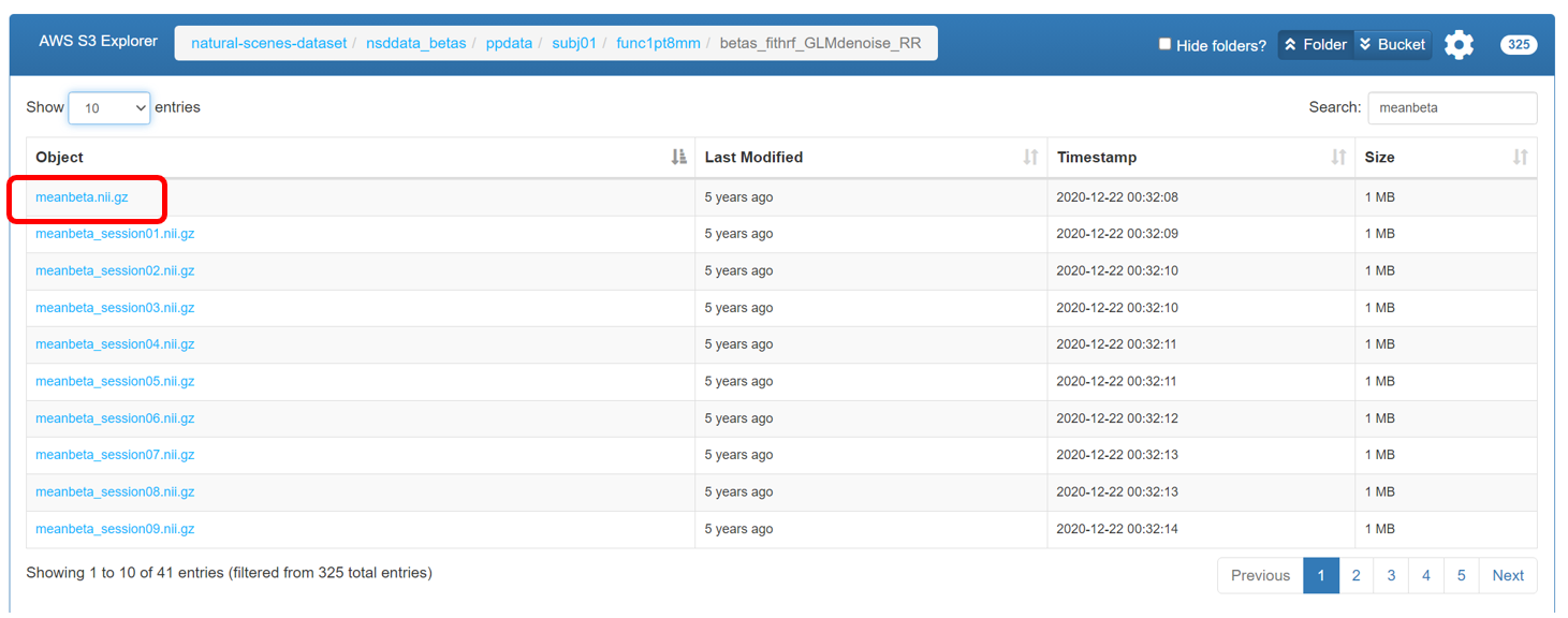

3. Once the files from the first two steps are downloaded to the server and the paths are correctly specified, you can run the following code to use Pycortex’s built-in functions to generate the database for each participant.

import cortex

for subj in range(1, 9):
    cortex.freesurfer.import_subj(f'subj0{subj}', pycortex_subject=f'subj0{subj}', freesurfer_subject_dir='/home/YOURNAME/freesurfer/subjects/', whitematter_surf='smoothwm')
    cortex.freesurfer.import_flat(f'subj0{subj}', 'full', hemis=['lh','rh'], cx_subject=f'subj0{subj}', flat_type='freesurfer', auto_overwrite=True, freesurfer_subject_dir='/home/YOURNAME/freesurfer/subjects/', clean=True)
    cortex.align.automatic(f'subj0{subj}', 'full', f"/YOURPATH/meanbeta.nii.gz")

Here is a brief explanation for the code:

• cortex.freesurfer.import_flat is used to import the surface data reconstructed by FreeSurfer (e.g., white matter, cortical thickness, curvature, etc.) into the Pycortex database.
• cortex.freesurfer.import_flat then imports FreeSurfer’s flatmap, which allows data to be displayed on a 2D unfolded cortical surface.
• cortex.align.automatic finally uses FreeSurfer’s boundary-based registration method to automatically align the functional data (in this case, meanbeta.nii.gz) to the subject’s anatomical surface. The resulting transformation is stored in the database and can be directly used to project the corresponding data onto the cortical surface for visualization.

1. After completing the above steps, you will find that under the path INSTALL_DATA/share/pycortex/, each participant’s database is generated. Here, for example, INSTALL_DATA corresponds to home/YOURNAME/anaconda3/envs/YOURVENV.

Of course, the exact location of the database can also be modified via the options.cfg file. The specific method is described here: Pycortex Documentaion: surface database. Simply speaking, you can find the filestore directory by running:

import cortex
cortex.database.default_filestore

Note: It is important to point out that the workflow described above does not have to strictly follow the example paths or the specific fMRI alignment reference files. You can customize the settings as long as the paths and references are consistent throughout. For example, in this demonstration, the reference file used is meanbeta.nii.gz located under func1pt8mm/betas_fithrf_GLMdenoise_RR/, which corresponds to a resolution of 1.8 mm. The NSD dataset also provides higher-resolution data (0.8 mm), which can be used depending on your specific requirements.

IV. Visualization Workflow

1. Core Visualization Code

Once we have all the prerequisite files, we can map the data onto the 2D cortex to generate a flatmap. Below is the complete code for visualization. The core functions, cortex.Volume and cortex.quickflat.make_figure, are also documented in detail on the official website: Pycortex Documentaion.

Here, data_to_project corresponds to the raw data to be mapped from the prerequisite files, while subject and xfm specify which surface database to use.

Note: The cmap parameter in cortex.Volume can be used to adjust the color scheme of the flatmap. A list of available colormaps can be found here: Pycortex Documentaion: colormaps. Personally, I like the magma colormap, and I hope everyone using Pycortex can find a color scheme they enjoy. 😊

import cortex
import numpy as np
import matplotlib.pyplot as plt

subject = f'subj0{subj}'
xfm = 'full'

# Creating the dataset that is the shape for this transform with one entry for each voxel
data_to_project = np.load("PATH_TO_SAVE_THE_DATA") 
data_to_project = np.swapaxes(data_to_project, 0, 2)

fig=plt.figure(figsize=(12, 6), dpi=300)

vol_data = cortex.Volume(test_data, subject, xfm, cmap="magma", vmin=0.0, vmax=0.6)

cortex.quickflat.make_figure(vol_data, with_curvature=True, with_sulci=True, nanmean=True, fig=fig, linewidth=3, labelsize="20pt",) 
fig.text(0.5, 0.13, "YOURMETRIC", fontsize=17, fontweight='bold', ha='center', va='center', transform=fig.transFigure)

plt.show()

2. ROI Labeling

After completing the steps above, we will find that the data can be perfectly visualized on the flatmap. However, the ROI annotations appear to be missing. An ROI (Region of Interest) refers to a specific brain region selected by the researcher for focused analysis or statistical evaluation of neural activity. So how do we annotate ROIs? Here, we need to use a tool called Inkscape, an open-source vector graphics editor that can be used to edit cortical ROI overlay files (overlays.svg), since these regions are stored in vector format.

Because the previous steps are performed on a remote server, using Inkscape for editing also requires XLaunch to forward the remote graphical interface to your local machine for operation.
Note: There are many online tutorials for installing Inkscape and XLaunch, so we will not cover the installation here. The XLaunch forwarding workflow can also be referred to in Section VI, Subsection 3.

Below is the specific code workflow for defining ROIs based on an existing surface database.

import cortex
import nibabel as nib
import numpy as np
import argparse

parser = argparse.ArgumentParser()
parser.add_argument("--roi_dir", type=str, default="YOURPATH")
parser.add_argument("--subj", type=int, default=1)
parser.add_argument("--xfm", type=str, default="full")
parser.add_argument("--rois", nargs="*", type=str, default=["prf-visualrois", "floc-places", "floc-bodies"])
args = parser.parse_args()

for roi in args.rois:
    roi_dat = nib.load(f"{args.roi_dir}/subj0{args.subj}/func1pt8mm/roi/{roi}.nii.gz")
    overlay_dat = roi_dat.get_fdata().swapaxes(0, 2)
    
    mask = overlay_dat > 0
    current_roi_data = np.where(mask, overlay_dat, 0)

    V = cortex.Volume(
        current_roi_data,
        f"subj0{args.subj}",
        args.xfm,
        mask=cortex.utils.get_cortical_mask(f"subj0{args.subj}", args.xfm),
        vmin=0,
        vmax=np.max(current_roi_data),
    )

    cortex.utils.add_roi(V, name=roi, open_inkscape=True, add_path=True, with_colorbar=True)

The files containing ROI information should be specified using --roi_dir. These ROI files are also available on AWS S3: natural-scene-dataset, specifically under the directory natural-scenes-dataset/nsddata/ppdata/subj0X/func1pt8mm/roi.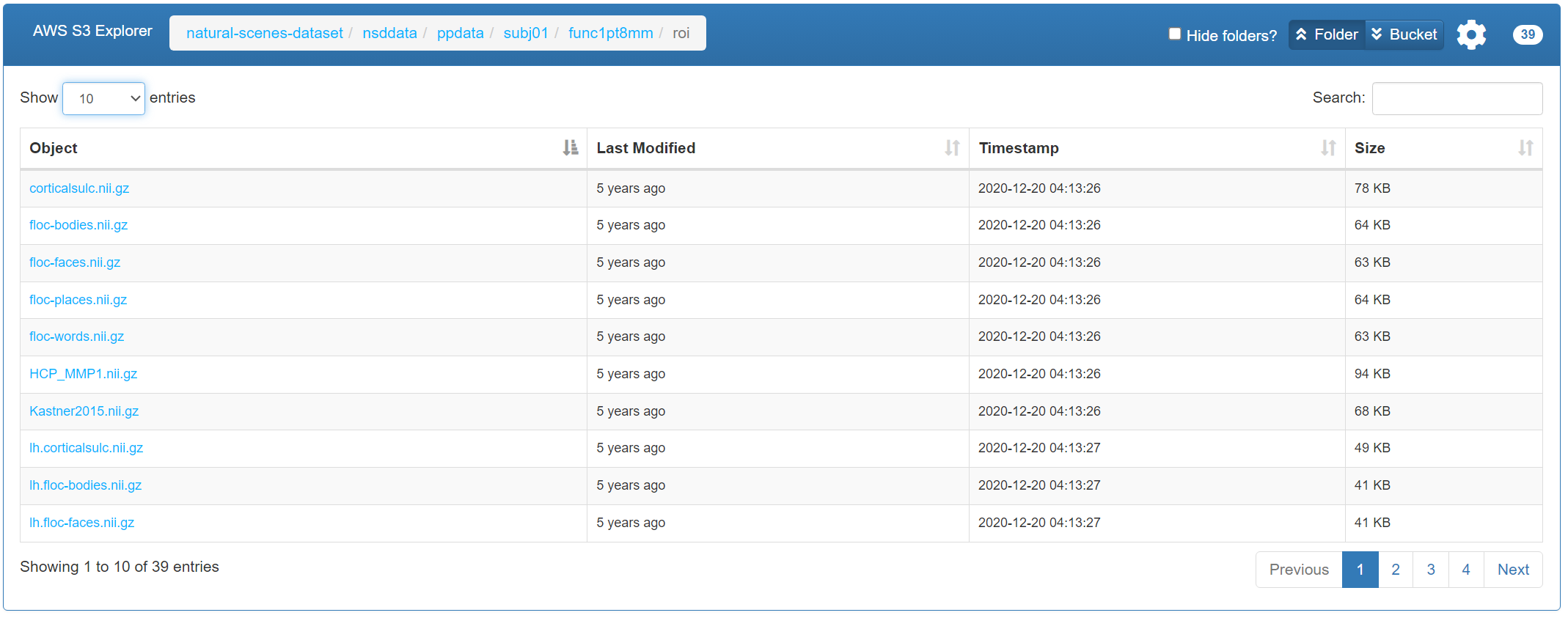

These ROI files contain annotation data for both the cortical surface and volumetric space. The size of the ROI data matches the voxel data, i.e., (H, W, B). Each value in the ROI data represents the label of the corresponding voxel: -1 indicates a non-cortical voxel, 0 indicates an unlabelled voxel, and positive integers indicate specific ROI IDs. For more details, please refer to NSD: ROI.

For example, the floc-places ROI template includes regions OPA, PPA, and RSC, so the positive integer labels are {1, 2, 3}. In code, we can use mask = overlay_dat > 0 to obtain the ROI regions corresponding to this template. When performing boundary annotation in Inkscape, the voxels are displayed in colors distinct from the background. Since different ROIs have different positive integer labels, they are displayed in different colors, allowing for clear differentiation between ROI regions.

During the ROI annotation workflow, the Inkscape interactive interface will appear. You can select the Freehand Line tool from the left panel and draw along the borders of the ROI. After finishing, save and close the interface.

In the example code, this process is executed in a loop over three templates: "prf-visualrois", "floc-places", and "floc-bodies". If you want to annotate more ROIs, refer to NSD: ROI. The next template will automatically appear for annotation, and the process is repeated until the loop is finished.

For a more detailed guide on annotating ROIs using Inkscape, see Drawing ROIs in Inkscape for Pycortex. 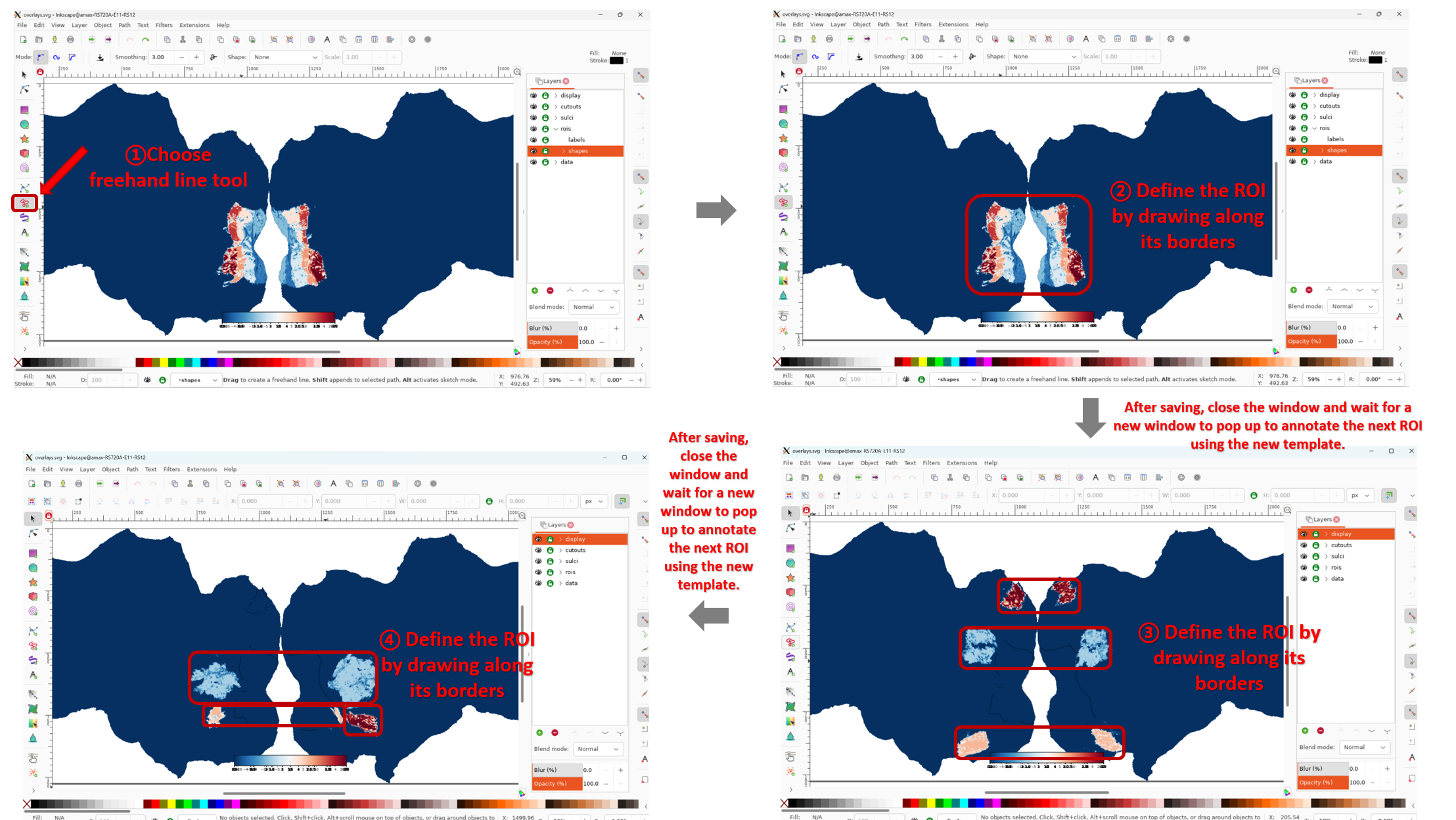Note: The above describes the general workflow for annotating ROIs. However, if you want to assign names to each ROI, you need to open the ROIs panel on the right and manually enter the name for the currently annotated ROI.

Finally, after completing the ROI annotations, you can re-run the core visualization code from Section 4, and you will see that the flatmap now includes the ROI labels.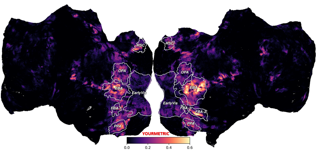

V. Public Release of the NSD Dataset Surface Database

Since the entire process of extracting the surface database can be somewhat complex, I also provide the surface databases for all 8 NSD participants, where the overlays.svg files already include ROI annotations, making Pycortex visualization more convenient.

Surface database link: AbabababaSmart: Pycortex_surface_database_for_NSD.

Once you have obtained each participant’s database, you can place them directly into the default directory INSTALL_DATA/share/pycortex/. Then, by running the core visualization code from Section 4, you can generate flatmap visualizations of the data projected onto the 2D cortex, with the ROI regions already delineated.

Note: The ROI annotations provided here are relatively coarse and mainly rely on templates such as prf-visualrois, floc-places, and floc-bodies. For more refined ROI definitions, please refer to the ROI annotation workflow in Section 4. For all ROIs that can be defined in the NSD dataset, see NSD: ROI.

VI. Common Issues

1. Flatmap Rotated by 90°

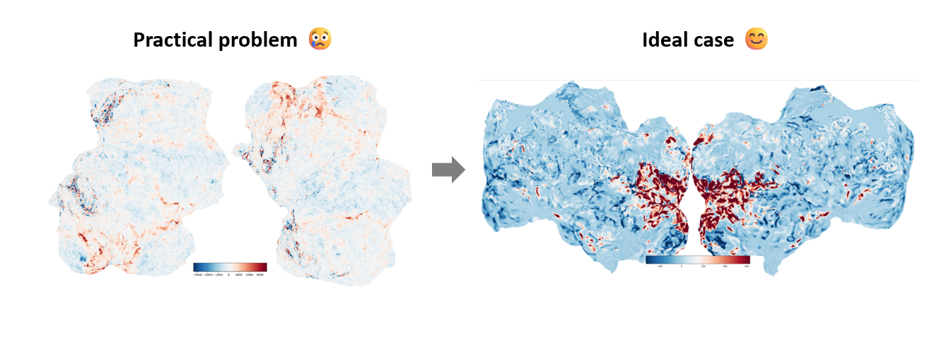
Some users may encounter the issue of the flatmap being rotated by 90°, as shown in the left figure above. The exact cause is currently unknown. However, the solution is very simple: it only requires modifying a small part of the Pycortex source code.

Specifically, you need to locate the file cortex.freesurfer.py and modify the following part of the code:

for hemi in hemis:
        if flat_type == 'freesurfer':
            pts, polys, _ = get_surf(fs_subject, hemi, "patch", patch+".flat", freesurfer_subject_dir=freesurfer_subject_dir)
            # Reorder axes: X, Y, Z instead of Y, X, Z
            # flat = pts[:, [1, 0, 2]] 
            # Flip Y axis upside down
            # flat[:, 1] = -flat[:, 1] 
            flat=pts 

Finally, you will obtain a normal flatmap as shown in the right figure. For a detailed discussion and other possible solutions, see https://github.com/gallantlab/pycortex/issues/488.

2. Flatmap Sulcus/Gyrus Settings

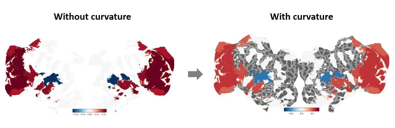
During flatmap visualization, if cortical curvature information (i.e., the folds and gyri of the brain) is not set, regions without data may blend into the white background.

To display cortical curvature on the flatmap, simply ensure that in the core visualization code from Section 4, you pass the parameters with_curvature=True and with_sulci=True to cortex.quickflat.make_figure.

• with_curvature=True displays the gyri and sulci in grayscale to show the convex and concave structures.
• with_sulci=True draws lines indicating the locations of the sulci.

3. Defining ROIs with Inkscape via XLaunch

Below we also provide an optional step-by-step procedure that documents an alternative, successful XLaunch forwarding workflow. The following command $env:DISPLAY = "localhost:{display number}" should be executed in your local terminal window. Then, after SSH-ing into the remote server, you can run the ROI annotation code.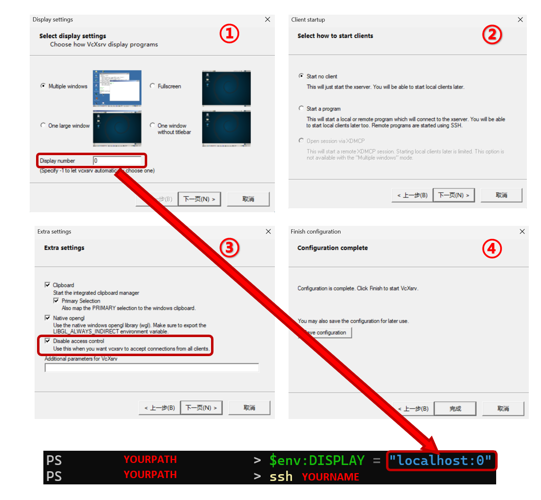

4. Visualization Methods for Other Datasets Beyond NSD

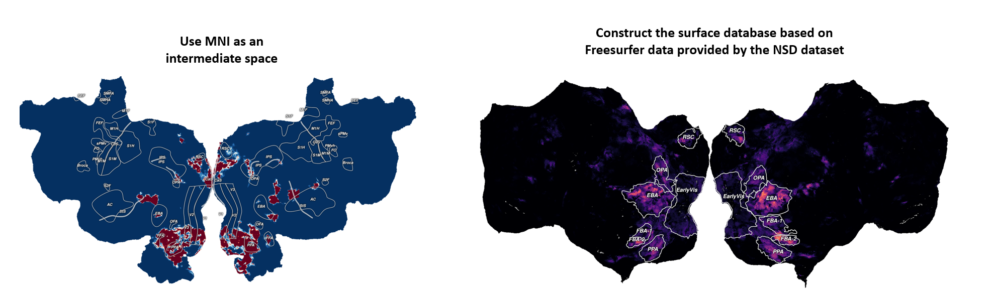
This tutorial mainly documents the method for visualizing the NSD dataset using Pycortex. However, for other datasets, the visualization method may vary depending on the dataset.

One method inherited from our lab is based on the core idea of using MNI space as an intermediate standardized coordinate system. The steps are as follows:

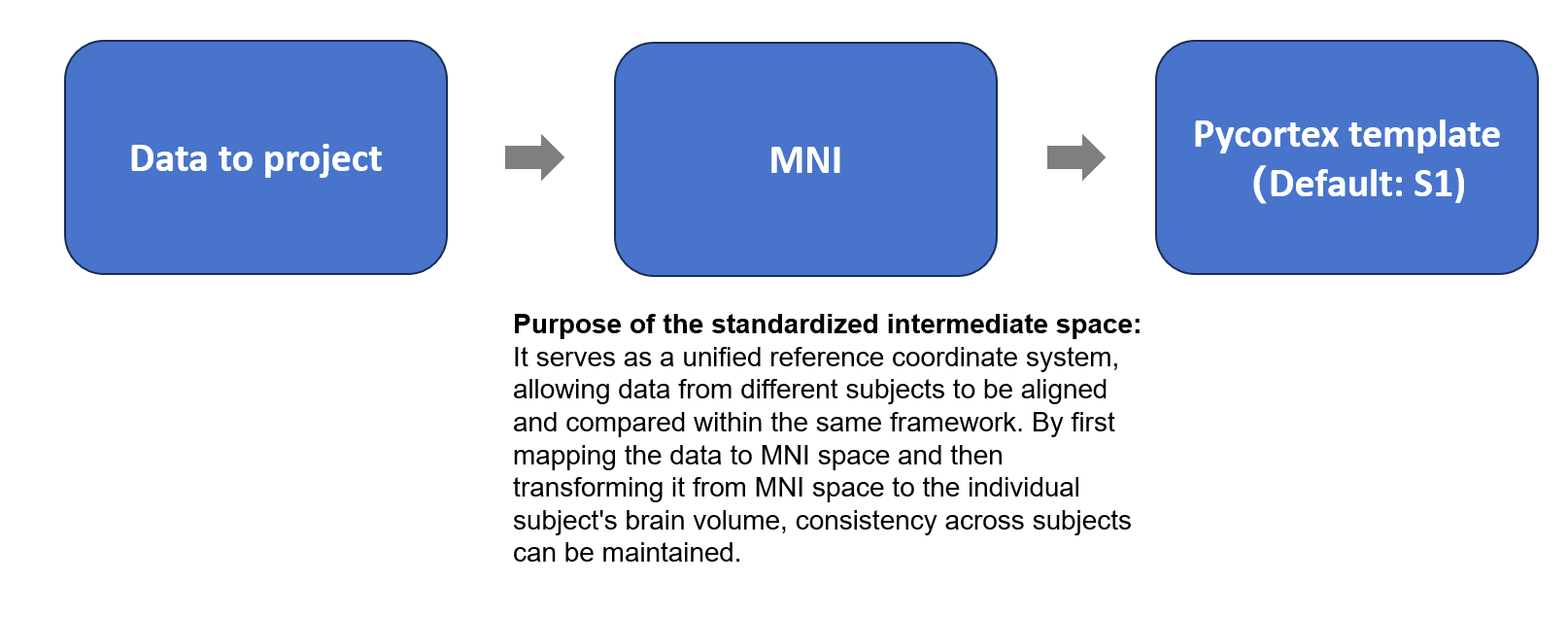
1. Align the data to be projected to the MNI template and resample it to ensure voxel correspondence.
2. Use the precomputed transformation from MNI space to the Pycortex template subject space (S1) to map the data to the individual brain volume.
3. Finally, visualize the data on Pycortex’s flatmap.

Note: Here, Pycortex provides a default surface database named S1, which also includes ROI annotations.

The code workflow is as follows. data_to_project.nii.gz is the data to be projected. MNI152_T1_1mm_Brain.nii.gz is a standardized brain template generated by averaging the T1-weighted MRI scans of 152 healthy adults. This open-source template is easy to find online (download link). Of course, the standardized brain template does not have to be MNI152_T1_1mm_Brain.nii.gz; other templates can be used according to your needs.

import cortex
from cortex import mni
import nibabel as nib
from nilearn.image import resample_to_img

# Compute transformation from MNI space to subject S1
s1_to_mni = mni.compute_mni_transform(subject='S1', xfm='fullhead', template="MNI152_T1_1mm_Brain.nii.gz")

# Load the template and the data to project
img1 = nib.load("MNI152_T1_1mm_Brain.nii.gz")
img2 = nib.load("data_to_project.nii.gz")

# Resample the data to match the template voxels
img2_resampled = resample_to_img(img2, img1, interpolation="nearest")
img2_resampled_data = img2_resampled.get_fdata()

# Project the MNI data into the subject S1 space
new_sub_data = mni.transform_mni_to_subject('S1', 'fullhead',
                                            img2_resampled_data, s1_to_mni, template="MNI152_T1_1mm_Brain.nii.gz")

# Save the subject-space data
nib.save(new_sub_data, "mni_to_sub.nii.gz")

import matplotlib.pyplot as plt

# Create a Pycortex Volume object and plot the flatmap
fig = plt.figure(figsize=(10,8))
volume = cortex.Volume("mni_to_sub.nii.gz", 'S1', 'fullhead')
cortex.quickflat.make_figure(volume, with_curvature=True, with_sulci=True, fig=fig)

Note: Although this method is inherited from our lab, its visualization accuracy remains to be validated. When tested using the NSD dataset, the projected positions show some deviations, which may be due to factors such as template selection, individual anatomical differences, transformation precision, and resampling errors. Moreover, I do not fully understand every step of the transformations involved. Therefore, I encourage readers to consult the transformation data provided by the dataset itself to ensure more accurate flatmap visualizations.

Reference

[1] A massive 7T fMRI dataset to bridge cognitive neuroscience and artificial intelligence | Nature Neuroscience
[2] Natural Scenes Dataset Website
[3] NSD Data Manual - Slite
[4] Pycortex Documentation
[5] Drawing ROIs in Inkscape for Pycortex
[6] Github: pycortex/issues/488
[7] Using Linux with GUI on Windows 11 (WSL, SSH, Remote Desktop …) | by Elim Kwan | Medium
[8] Github: MNITemplate

Final Remarks

This concludes the workflow for visualizing the NSD dataset using Pycortex. Although the description here may appear quite detailed, it is possible that some steps have been unnecessarily complicated and may not represent the most optimal solution. Therefore, if any readers are aware of more concise and efficient approaches, feedback and corrections are warmly welcomed.

Updated on September 25, 2025, on a gloomy rainy day. 🌧